Tutorial: strain clustering

Using gempipe derive, we generated GSMMs for 45 randomly picked strains belonging to 3 species of Lacticaseibacillus: L. casei, L. paracasei, L. rhamnosus (15 each). During the process, the binary feature table rpam.csv was generated, showing the presence / absence of metabolic reactions in each strain. Moreover, since we run gempipe derive with the options --cnps and --aux, two other binary feature tables were produced: cnps.csv and aux.csv. The first include the ability / inability of strains in catabolizing alternative C, N, P and S sources; the second report the presence / absence of auxotrophies for specific amino acids and vitamins.

These tables have always the same structure: binary metabolic features in row, strains (genome accessions) in column. As the features are binary, cells contain either 1 (feature present) or 0 (feature absent). Below we see the table for alternative substrates (cnps.csv): IDs are preceded by the source type (C, N, P or S), and substrates can be repeated if they are considered source of multiple types of atoms at the same time (for example, methionine met__L, having chemical formula C5H11NO2S, will be tested as C, N and S source, so it will appear in three separated rows).

import pandas as pnd

aux = pnd.read_csv('tutoring_materials/lacticaseibacillus/aux.csv', index_col=0)
cnps = pnd.read_csv('tutoring_materials/lacticaseibacillus/cnps.csv', index_col=0)
rpam = pnd.read_csv('tutoring_materials/lacticaseibacillus/rpam.csv', index_col=0)

cnps

	GCA_025190575.1	GCA_000026525.1	GCA_005864085.1	GCA_001013375.1	GCA_024329605.1	GCA_959021285.1	GCA_000311965.1	GCA_024329385.1	GCA_025190605.1	GCA_026427555.1	...	GCA_002091975.1	GCA_007989685.1	GCA_030224505.1	GCA_000735255.1	GCA_030480425.1	GCA_032466035.1	GCA_030215365.1	GCA_030361365.1	GCA_028578865.1	GCA_002091995.1
[C]melib	1	1	1	1	1	1	1	1	1	1	...	1	1	1	1	1	1	1	1	1	1
[C]Larab	0	0	0	0	0	0	0	0	0	0	...	0	0	0	0	0	0	0	0	0	0
[C]acald	1	0	0	1	0	0	0	1	1	0	...	1	0	0	0	1	0	0	0	0	0
[C]serglugly	0	0	0	0	0	0	0	0	0	0	...	0	0	0	0	0	0	0	0	0	0
[C]pacald	0	0	0	0	0	0	0	0	0	0	...	0	0	0	0	0	0	0	0	0	0
...	...	...	...	...	...	...	...	...	...	...	...	...	...	...	...	...	...	...	...	...	...
[S]met__L	1	1	1	0	1	0	1	1	0	0	...	1	0	0	0	0	0	0	1	0	0
[S]h2s	0	0	0	0	0	0	0	0	0	0	...	0	0	0	0	0	0	0	0	0	0
[S]gly_met	1	1	1	0	1	0	1	1	0	0	...	1	0	0	0	0	0	0	1	0	0
[S]taur	0	0	0	0	0	0	0	0	0	0	...	0	0	0	0	0	0	0	0	0	0
[S]methal_	0	0	0	0	0	0	0	0	0	0	...	0	0	0	0	0	0	0	0	0	0

307 rows × 45 columns

Now we try to build a dendrogram using all these binary metabolic features. We call such dendrogram a “phylometabolic tree”, as it resembles a phylogenetic tree, but it is built by using exclusively metabolic features. Then, we split this tree into clusters, which groups metabolically homogeneous strains together.

The assigned data-driven cluster can be compared with a strain-specific metadata such as the isolation niche or, like in this tutorial, the species of origin. This metadata is provided by one of the gempipe derive outputs, namely derive_strains.csv, which also summarizes reconstruction metrics and basic growth simulations before and after the strain-specific gap-filling phase:

report = pnd.read_csv('tutoring_materials/lacticaseibacillus/derive_strains.csv', index_col=0)
report.head()

	species	strain	niche	G	R	M	obj_value	status	R.1	inserted_rids	solver_error	obj_value_gf	status_gf
accession
GCA_008868595.1	Lacticaseibacillus casei	BIO5773	-	1039	1312	1212	0.0	optimal	1313	{'cdm25_gempipe': ['GLUR']}	-	{'cdm25_gempipe': 1.6898873415546019}	{'cdm25_gempipe': 'optimal'}
GCA_005864085.1	Lacticaseibacillus casei	FAM 20446	-	948	1255	1212	0.0	optimal	1256	{'cdm25_gempipe': ['ALATA_D']}	-	{'cdm25_gempipe': 1.6898873415543527}	{'cdm25_gempipe': 'optimal'}
GCA_018363095.1	Lacticaseibacillus casei	FBL6	-	1018	1289	1212	0.0	optimal	1290	{'cdm25_gempipe': ['GLUR']}	-	{'cdm25_gempipe': 1.6898873415546252}	{'cdm25_gempipe': 'optimal'}
GCA_002091995.1	Lacticaseibacillus casei	GCRL 163	-	1039	1265	1212	0.0	optimal	1266	{'cdm25_gempipe': ['GLUR']}	-	{'cdm25_gempipe': 1.7027403931953289}	{'cdm25_gempipe': 'optimal'}
GCA_037901485.1	Lacticaseibacillus casei	LC130	-	877	1229	1212	0.0	optimal	1230	{'cdm25_gempipe': ['GLUR']}	-	{'cdm25_gempipe': 1.1298198948419083}	{'cdm25_gempipe': 'optimal'}

Now we have all the necessary inputs for building the phylometabolic tree, splitting the tree into data-driven clusters, and comparing clusters with a biologically relevant metadata.

First of all, the phylometabolic tree must be built, and the strains assigned to clusters. To this aim, we use the gempipe.silhouette_analysis function, which performs a Silhouette analysis. This evaluates the quality of clustering by measuring how well each data point fits within its own cluster compared to neighboring clusters. The Silhouette Coefficient quantifies the cohesion and separation of individual data points, ranging from -1 (misclassified) to +1 (well-clustered), providing insight into the suitability of cluster assignments. The Average Silhouette Score, calculated across all data points, gives an overall measure of the clustering efficacy, helping identify optimal cluster numbers and detect poorly formed clusters.

In the range considered (ctotest), the Average Silhouette score have a peak at 4, but higher values can be reached: to avoid the risk of everfitting, and to work with a manageable number of clusters, we extract 4 clusters (forcen).

💡 Tip! Binary metabolic features can be thought as divided in “layers”: in this example we have 3 layers (reactions, auxotrophies, alternative substrates). However, the Gempipe API can manage any number of layers at the same time (tables): for example, it would be possible to add layers derived from “classic genomics”, indicating the presence/absence of key/marker genes.

To compare data-driven clusters with the species of origin (and not with the environmental niche), we use report_key='species'. Doing so, clusetering appears mostly concordant with the species of origin:

import gempipe

fig, acc_to_cluster, cluster_to_color = gempipe.silhouette_analysis(
    derive_report=report, report_key='species',
    tables={'auxotrophies': aux, 'C/N/P/S substrates': cnps, 'reactions': rpam},
    ctotest=range(2,31,1), forcen=4, 
    outfile='tutoring_materials/lacticaseibacillus/silhouette_analysis.png',
)

WARNING: auxotrophies: replacing NA values for the following rows: {'[aux]cbl1', '[aux]pydx', '[aux]ascb__L'}.

Now, the phylometabolic tree can also be represented as a “heatmap” (or, better, a presence/absence matrix using a different color for each layer of binary feature): to do so, we use the gempipe.heatmap_multilayer function, specifying the same layers and two dictionaries created by the previous function: accession-to-cluster and cluster-to-color.

fig, ord_data_bool = gempipe.heatmap_multilayer(
    derive_report=report, report_key='species',
    tables = {'auxotrophies': aux, 'C/N/P/S substrates': cnps, 'reactions': rpam},
    acc_to_cluster=acc_to_cluster, cluster_to_color=cluster_to_color,
    outfile='tutoring_materials/lacticaseibacillus/phylomet_dendro.png')

WARNING: auxotrophies: replacing NA values for the following rows: {'[aux]cbl1', '[aux]pydx', '[aux]ascb__L'}.

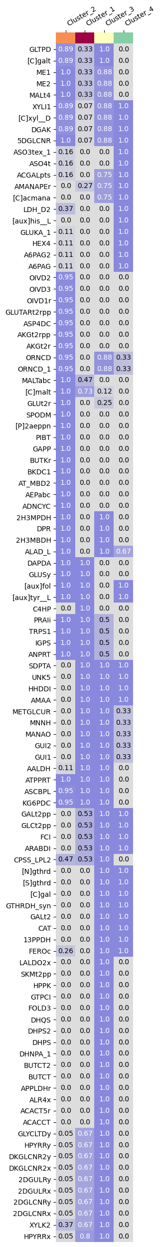
With the above figure, it is evident that specific features are characterizing clusters. But which features? To extract the most discriminative features, we use the gempipe.discriminant_feat function. This plots the features consistently present or absent in at least a cluster, meaning that their relative frequency of presence is ≥0.90 or ≤0.10 in a cluster.

Features are named as in their original tables (in this case, rpam.csv, cnps.csv and aux.csv). Therefore, features without prefixes ([C], [N], [P], [S] or [aux]) are simply modeled reactions, so they can be visualized on an Escher map. To give some examples, looking at [C]xyl__D we see that strains in Cluster_1 are mostly uncapable of utilizing xylitol as alternative C source; strains in Cluster_4 are consistently auxotroph for histidine ([aux]his__L), while strains in Cluster_3 are characterized by a self-production of folate ([aux]fol); strains in Cluster_2 are the only able to directly convert aspartate into alanine, having an aspartate 4-decarboxylase (ASP4DC).

Please note that these analysis are highly dependant on:

• the accuracy and completeness of the draft pan-GSMM given in input to gempipe derive (which in turn determines the accuracy and completeness of the strain-specific GSMMs);

• the number of genomes included in the analysis (in this tutorial as little as 45).

fig, df_relfreq = gempipe.discriminant_feat(ord_data_bool, acc_to_cluster, cluster_to_color)